What happens inside the simulation after CO₂ emissions stop?
A UK Earth System Model study finds that the temperature response after CO₂ emissions stop depends on prior warming. A two-tank example helps explain the difference between changing an input and resetting a system.

Stopping an input does not reset a state
Turn off a heater and the room does not instantly return to its earlier temperature. The walls, furniture and air have histories. The analogy is incomplete for Earth's climate, but it introduces an important programming idea: a system's current state contains consequences of earlier inputs. Setting tomorrow's input to zero is different from setting the whole system back to zero.
A study published in Nature Climate Change on 3 November tests this question with UK Earth System Model simulations. Human-caused CO₂ emissions stop at different starting warming levels. The researchers report little additional warming at starting levels up to 2°C, but a positive temperature commitment at higher levels, reaching about 0.4 to 0.6°C after roughly 150 years in those simulations. These are results from idealized experiments with a particular model, not a forecast for every emissions pathway.
The explanation involves both heat and carbon. Continued carbon uptake can reduce atmospheric CO₂ and exert a cooling influence, while the climate system is still adjusting to its energy imbalance. The balance changes with the starting conditions. The authors also use a simpler two-layer model to help explain the response. Our smaller example below isolates state and energy accounting; it does not model the carbon cycle or reproduce their findings.
Source: Zero emissions commitment depends on warming level, published 3 November
A smaller model can reveal the bookkeeping
For an original numerical illustration, imagine two connected tanks holding heat. The first exchanges heat with the outside; the second responds more slowly. At each time step, the program computes the transfer between them and any energy entering or leaving the pair. The numbers are invented for teaching and are not a reduced reproduction of the paper's climate experiment.
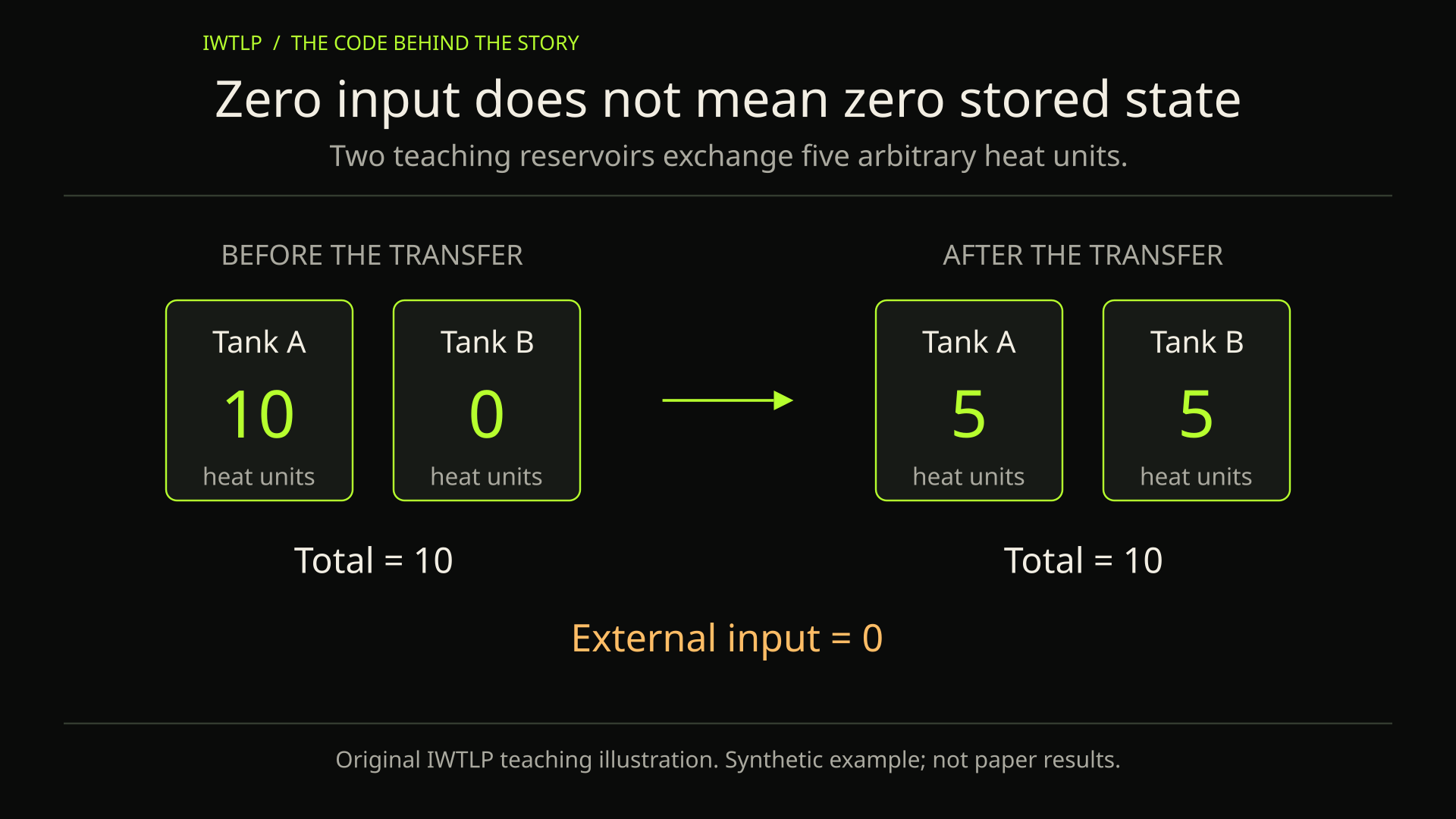
Suppose five arbitrary heat units leave the first tank for the second during one step. Subtract five from one and add five to the other. The total has not changed because of that internal transfer. This simple accounting check is powerful: if the code subtracts five twice, a graph may still look smooth while the model quietly destroys energy.
Now remove the external input while leaving the tanks' stored values untouched. The first tank can continue changing as heat moves between the two. Compare that run with a second experiment that incorrectly empties both tanks at the stopping time. They answer different questions. The difference is visible directly in the saved state, without needing a sophisticated visualization.
Compare scenarios at the same point in the story
A scenario comparison needs an explicit clock. One run might stop receiving input earlier than another. Aligning both curves only by their original start date can obscure what happened after the intervention. For our tank exercise, save the intervention time and produce a second time coordinate measuring elapsed steps since that event. Keep the original time coordinate as well.
Also distinguish an absolute value from a change relative to a baseline. A tank beginning at a higher stored value can remain higher even while cooling more quickly. Labeling a plotted difference requires naming which starting value was subtracted. In a climate analysis, the precise reference and averaging window belong with the result, rather than being reconstructed from a caption later.
The new study uses both a large Earth-system model and a simpler explanatory model. That pairing is valuable because different tools can answer different questions: one represents a richer interacting system, while another helps expose particular mechanisms. Agreement on one feature would not establish that the simpler model reproduces every regional or long-term behavior of the larger one.
Source: Study design and distinction between Earth-system simulations and emulations
Reproducibility starts with a small, complete question
The authors make processed diagnostics and figure-reproduction code available, while access arrangements differ for the full simulation output. That is an important practical distinction. Reproducing an analysis from saved diagnostics and rerunning the original Earth-system simulation are separate undertakings with different data and computing requirements.
For a first project, choose one published diagnostic and identify its units, scenario and averaging window. Then reproduce one transformation from the saved data. If two plots disagree, compare those choices before changing the model. Learning to track a temperature result back to its inputs gives you a practical starting point for reading larger climate studies.